The Simulation With Balls

Simulating the scoring system of The Quiz With Balls to understand if it is fair.

Introduction

 

In May 2024, Fox began airing The Quiz With Balls. The show features two teams of five competing in lighthearted trivia questions. The gimmick of the show is that any contestant who answers incorrectly is knocked into a pool of water by one the titular balls. Points escalate each round, and the family with the most points after five rounds gets to play for $100,000.

The show itself is kind of interesting, but the scoring is strange. My mathematical gut was telling me that the first round should very often determine the outcome of the entire game. Thus began my deep dive into the scoring and probability of The Quiz With Balls.

As a teaser, the scoring of The Quiz With Balls allows you to turn off your TV after the first round more than 25% of the time because you will already know the winner. Sometimes you will know with more than 90% certainty after the first round!

How The Quiz With Balls Works

Before diving into the math, I need to explain how The Quiz With Balls works.

There are two teams of five. I’ll call the teams \(A\) and \(B\). There are up to five rounds. Each round has two essentially identical stages. In stage one of round one, team \(A\) chooses one of ten categories. The categories broadly indicate the subject of the question, but are not specific enough to credibly inform contestants. Once team \(A\) has chosen their category, they are presented with the question. The question always has 6 options and as many correct answers as players remaining in that team. So at the start of the game, there are still 5 players on team \(A\), so there will be 6 possible answers 5 of which are correct.

Team \(A\) must then decide to assign their 5 contestants into 5 of the 6 possible options. Players may not double-up on the same answer or choose to sit out. Players walk into a slot corresponding to their selected answer. Then the correct answers are revealed by six balls rolling down the slots. If an answer is correct, the ball stops just before hitting the contestant. If an answer is incorrect, the ball rolls into the player, knocking them into the pool, and removing them from the rest of the game. So if team \(A\) gets an incorrect answer in the first round, they will start the next round with \(4\) players. There is no mechanism for players to return to the team once they have been knocked into the pool.

The second stage of round one is for team \(B\). They select one of the nine remaining categories, they are given the question, they assign their five players to five slots, and then the balls reveal which answer was correct.

Then, in round 2 the game proceeds as before, but now with as many correct answers as remaining players. For example, if there are 4 players remaining on team \(A\), and the question is: “Which of the following are shades of red?” You may have answers like:

1. Carmine ■
2. Chartreuse ■
3. Maize ■
4. Salmon ■
5. Scarlet ■
6. Vermilion ■

The boldface answers are correct.¹ Since there were four players remaining, there were four correct answers. (Of course, the contestants would not see the boldfacing or the colored blocks).

Play continues until 5 rounds have elapsed or one team loses all of its players.

Scoring is cumulative between rounds, and the number of points in round \(t\) is equal to \(\$1,000\) times \(t\) times the number of correct answers in that round. So 3 correct answers in round 4 would give \(\$1,000\cdot4\cdot3=\$12,000\).

The team with the most points at the end of round 5 then plays a minigame for the chance to win \(\$100,000\). I will not model this final round because I am more interested in the competition between the two teams.

Modeling The Quiz With Balls

In this section, I will model the probability of a team going from one number of players in round \(t\) to another number of players in round \(t+1\).

Suppose that there are \(b\) total balls² and \(p\) remaining players in round \(t\). The host will then generate a question with \(p\) correct answers, one for each player. We want to determine the probability that \(j\) players get the question correct given that there are \(p\) remaining players and \(b\) possible options.³ If \(j\) players get the question correct, then \(j\) players advance to the next round.

The easiest way to proceed is to break the probability into something like:

\[ \frac{\# \text{ of ways to get }j\text{ correct}}{\# \text{ of total outcomes}} \]

The numerator is a little challenging, but it can be split into three subproblems:

1. How many ways are there to choose which of the \(p\) are in the \(j\) correct slots?
2. Within the correct \(j\) players, how many ways are there to allocate them into the \(p\) correct slots (since there are always \(p\) correct answers)?
3. Within the incorrect \(p-j\) players, how many ways are there to allocate them into the \(b-p\) incorrect slots.

There is a subtle difference between the first question and the latter two. In the first question, we do not care about the actual ordering of the players within their group, we only care about who will respond correctly (not which answer they will respond to). In the latter two questions, we are able to use our knowledge of who is in each group to ask where each person will be allocated. So for the first question, we do not care about ordering, but in the latter two, we do care about ordering.

Also, you may be asking why we don’t have to answer a question like: “How many ways are there to choose which players in the incorrect slots?” We do not need to determine that quantity because it is always exactly determined by the people who get the question correct. Since there are only two categories, once you have chosen the correct players, then all of the other players fall into the incorrect bin. So this question would not introduce any new scenarios.

Starting with question 1., this is simply the number of ways to choose \(j\) players from \(p\) choices, so \(nCk(p,j)=\frac{p!}{j!(p-j)!}\). Since each player must be allocated to exactly one slot, we can use the combination formula.

For question 2., this is the number of ways to order \(j\) players within \(p\) slots, or \(nPk(p,j)=\frac{p!}{(p-j)!}\).

And finally, for question 3, we ask how many ways are there to order the \(p-j\) into \(b-p\) slots, so \(nPk(b-p, p-j)=\frac{(b-p)!}{((b-p)-(p-j))!}\). Notice that 1., 2., and 3. do not depend on each other, so the total number of ways to get \(j\) correct answers is the product of the three quantities.

So the total number of ways to get \(j\) correct given that you currently have \(p\) players is:

\[ \text{\# of ways for} \ j \ \text{correct answers} = \frac{p!}{j!(p-j)!} \cdot \frac{p!}{(p-j)!} \cdot \frac{(b-p)!}{((b-p)-(p-j))!} \]

Then, let’s tackle the denominator. Here we’re trying to count the total number of outcomes. Notice that the total number of ways to allocate \(p\) players in to \(b\) slots is \(nPk(b,p)=\frac{b!}{(b-p)!}\). So the probability of starting with \(p\) players, and getting \(j\) correct answers is:

\[ f(j,p,b)=\frac{\frac{p!}{j!(p-j)!} \cdot \frac{p!}{(p-j)!} \cdot \frac{(b-p)!}{((b-p)-(p-j))!}}{\frac{b!}{(b-p)!}} \]

This expression does not simplify nicely, so we will use \(nPk\) and \(nCk\) directly when computing probabilities. Despite the relative inelegance of the above expression, it turns out to be quite powerful when modeling The Quiz With Balls. Now, we are able to take any game state (the current number of remaining players), and predict the distribution of game states in the next period.

Let’s implement this function \(f\) in python:

import numpy as np
import math

# Create a version of nPk that doesn't do more computation than necessary
def nPk(n: int, k: int) -> int:
  # uses a ternary expression to return 0 if trying to choose more than available
  return np.prod(range(n-k+1,n+1)) if k<=n else 0

def f(j: int, p: int, b: int) -> float:
  numerator = math.comb(p,j) * nPk(p, j) * nPk(b-p,p-j)
  denominator = nPk(b,p)
  return (numerator/denominator)

f(4,5,6)

The last line of the above says that the probability of getting 4 correct answers when you have 5 players and 6 balls is 83%.

This function \(f\) allows us to consider the probability of going from any number of players \(p\), to any number of correct answers \(j\).

Win Probability

Even with all of this technology, it is difficult to exactly compute the probability that a team will win given certain conditions. Getting win probabilities essentially requires us to determine the probabilities of certain point totals. Point totals are very difficult to reason about because they depend on both the number of correct answers and the rounds in which those answers took place (since points escalate each round). For example, a team that has the sequence of number of correct answers \(5,4,2,2\) has the same point total as a team that has a sequence \(4,3,3,2\) when you account for escalating point values.

But we’re not completely without hope, even if we can’t compute the ex ante probabilities of certain point totals, we can easily compute the point total of any given sequence of outcomes. And since we can easily predict the probability of going from one state to another, we can simulate many games, and empirically determine win probabilities given certain conditions.

Below, I construct a python class outlining how a team can play in The Quiz With Balls. I then create a class to describe how multiple teams play a game. The details aren’t essential, this just allows me to quickly simulate many games. I have “folded” the code, but feel free to take a look if you are interested.

from string import ascii_uppercase
from numpy.random import choice
import pandas as pd

class Team:
  
  def __init__(self, n_balls: int, name: str = None):
    
    self.finished = False
    
    self.n_balls = n_balls
    
    self.name = name
    if self.name is None:
      # if no name was given, make it a random string
      self.name = ''.join(choice(ascii_uppercase) for i in range(6))
  
    self.players = self.n_balls - 1
    self.points = 0
  
    self.player_history = [self.players]
    self.point_history = [self.points]
    
    # for each combination of j and p, compute the probability
    x = [f(j,p,self.n_balls) for j in range(self.n_balls) for p in range(self.n_balls)]
    
    # convert the 1D array of probabilities to a matrix
    # and transpose so indexes are as expected
    self.M = np.reshape(x, (-1,self.n_balls)).T
  
  def play_round(self, round_number: int):
    
    # If not finished, run a simulation
    if not self.finished:
      probs = self.M[self.players, :]
      
      self.players = np.random.choice(range(self.n_balls),1,p=probs)[0]
      self.points += round_number * self.players
      # If you're ending the round with zero players, you're finished
      if self.players == 0:
        self.finished = True
    
    # Either way, append info to the history
    self.player_history.append(self.players)
    self.point_history.append(self.points)
      
    return (self.players, self.points)
  
  def rig_round(self, round_number, n_correct):
    assert self.players >= n_correct
    # If not finished, rig this round
    if not self.finished:
      
      self.players = n_correct
      self.points += round_number * self.players
      # If you're ending the round with zero players, you're finished
      if self.players == 0:
        self.finished = True
    
    # Either way, append info to the history
    self.player_history.append(self.players)
    self.point_history.append(self.points)
    
  def summarize(self):
    out = {
      'name' : self.name,
      'players': self.players,
      'points': self.points
      }
      
    return out

class Game:
  def __init__(self, n_balls=6, n_teams=2):
    assert n_teams <= 26 # needed for team naming
    self.n_balls = n_balls
    self.n_teams = n_teams
    self.finished = False
    self.round_number = 1
    self.winner = None
    self.teams = [Team(self.n_balls, name = ascii_uppercase[i]) for i in range(self.n_teams)]
    
  def is_finished(self):
    finished_teams = np.sum([t.finished for t in self.teams])
    one_remaining = finished_teams >= (self.n_teams - 1)
    out_of_turns = self.round_number > 5
    # The game is over as soon as there is only one team not 
    # finished
    return one_remaining | out_of_turns
  
  def play(self):
    
    #while self.finished is False:
    while not self.finished:
      # Keep playing until all teams are out
      [t.play_round(self.round_number) for t in self.teams]
      self.round_number += 1
      self.finished = self.is_finished()

    # Print score at end of game
    scores = [t.points for t in self.teams]
    
    # Test to see if it's not a tie
    if any(scores[0]!=scores[1:]):
      self.winner = np.argmax(scores)
      return None
  
  def summarize_game(self):
    x = [t.summarize() for t in self.teams]
    df = pd.DataFrame(x)
    df['won'] = [self.winner == i for i, _ in enumerate(self.teams)]
    df['round'] = self.round_number
    return df
    

def simulate(n: int = 10000, WorkingGame = Game):
  summaries = []
  for i in range(n):
    g = WorkingGame()
    g.play()
    df = g.summarize_game()
    df['game_no'] = i
    summaries.append(df)
    
  df = pd.concat(summaries)
  # make sure index isn't duplicated
  df = df.reset_index(drop = True)
  
  df['rigging'] = WorkingGame.__name__

  return df

Baseline Results

Now, we have everything we need to simulate The Quiz With Balls. I am interested in how the results of the first round determine the rest of the game, but to make sure that everything is working as expected, let’s simulate 10,000 games completely randomly.

np.random.seed(0)
df = simulate(n=10000)

df.to_csv('unfavored.csv', index = False)

Here, since we started symmetrically, we should expect teams \(A\) and \(B\) to win a roughly equal number of games. Below I plot the simulated fraction of games won by team \(A\) and team \(B\).

library(ggplot2)
library(ggchameleon)

library(dplyr)

df <- read.csv('unfavored.csv') 
win_counts <- 
  df |> 
  summarize(winner = case_when(
    any(name=="A" & won=='True') ~ "A Wins",
    any(name=="B" & won=='True') ~ "B Wins",
    T ~ "Tie"
  ),
  .by = game_no) |> 
  filter(winner!='Tie') |> 
  summarize(n = n(), .by = winner) |> 
  mutate(total = sum(n)) |> 
  rowwise() |> 
  mutate(ci = list(binom.test(n,total)$conf.int)) |> 
  mutate(ci_lower = ci[1],
         ci_upper = ci[2])

b_test <- binom.test(win_counts$n[1], win_counts$total[1])
p_val_fmt <- format(b_test$p.value, digits = 4)

# Only need to check the first test since they're actually the same
fail_to_reject <- all( (win_counts$ci_lower<=.5) & (win_counts$ci_upper>=.5) )
stopifnot(fail_to_reject)

n_sims <- nrow(df)/2
n_ties <- n_sims - win_counts$total[1]

gg <- 
  ggplot(win_counts)+
  geom_col(aes(x=winner, y =n/sum(n)))+
  geom_errorbar(aes(x=winner,ymin=ci_lower,ymax=ci_upper),width = 0.2)+
  ggtitle("Fraction of Games Won by Each Team",
          "95% Confidence Intervals of Winning Probability")+
  xlab(NULL)+
  ylab(NULL)+
  labs(caption = glue::glue("{n_ties}/{n_sims} simulations excluded due to ties"))

gg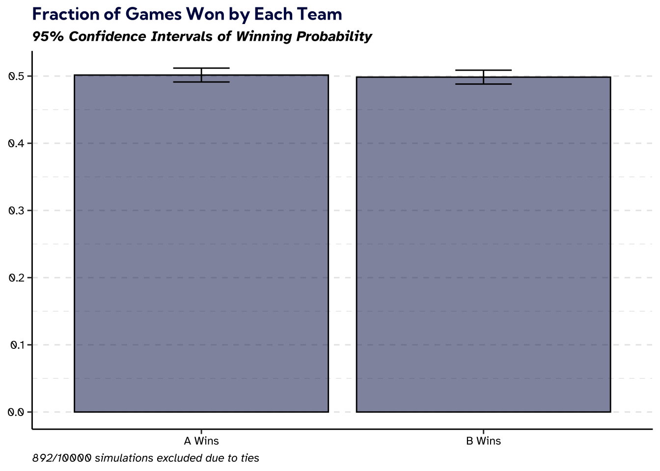

Since there is randomness in the games, the observed win probabilities are not exactly equal. However, a binomial test reveals that the win probabilities are not significantly different from each other (\(p\)-value 0.7772).

If Team \(A\) Wins the First Round

Finally, let’s tackle my initial question: if team \(A\) does better in the first round, what is the probability that they win the entire game? In particular, I will run another 10,000 simulations. Instead of starting at the beginning of the game, we will start each game in the second round. We will override the first round so that team \(A\) got all 5 correct, but team \(B\) lost a player, and only got 4 correct. Then we let the natural simulation dynamics play out for the rest of the game.

# Create a class inheriting from the standard game 
class FavorA(Game):
  def __init__(self):
    # Creates the unbiased game
    super().__init__()
    # Override the first round to favor A
    self.teams[0].rig_round(1,5)
    self.teams[1].rig_round(1,4)
    self.round_number = 2

# Run simulation favoring A
np.random.seed(1)
df = simulate(n=10000, WorkingGame = FavorA)

df.to_csv('favor_a.csv', index = False)

Reproducing the same plot from before, we have:

df <- read.csv('favor_a.csv')
win_counts <- 
  df |> 
  summarize(winner = case_when(
    any(name=="A" & won=='True') ~ "A Wins",
    any(name=="B" & won=='True') ~ "B Wins",
    T ~ "Tie"
  ),
  .by = game_no) |> 
  filter(winner!='Tie') |> 
  summarize(n = n(), .by = winner) |> 
  mutate(total = sum(n)) |> 
  rowwise() |> 
  mutate(ci = list(binom.test(n,total)$conf.int)) |> 
  mutate(ci_lower = ci[1],
         ci_upper = ci[2])

b_test <- binom.test(win_counts$n[1], win_counts$total[1], p = .9, alternative = "greater")
lower_bound <- format(b_test$conf.int[1]*100, digits = 4, scientific = F) 

# Only need to check the first test since they're actually the same
stopifnot(b_test$p.value<.05)

n_sims <- nrow(df)/2
n_ties <- n_sims - win_counts$total[1]

gg <- 
  ggplot(win_counts)+
  geom_col(aes(x=winner, y =n/sum(n)))+
  geom_errorbar(aes(x=winner,ymin=ci_lower,ymax=ci_upper),width = 0.2)+
  ggtitle("Fraction of Games Won by Each Team",
          "95% Confidence Intervals of Winning Probability")+
  xlab(NULL)+
  ylab(NULL)+
  labs(caption = glue::glue("{n_ties}/{n_sims} simulations excluded due to ties"))

gg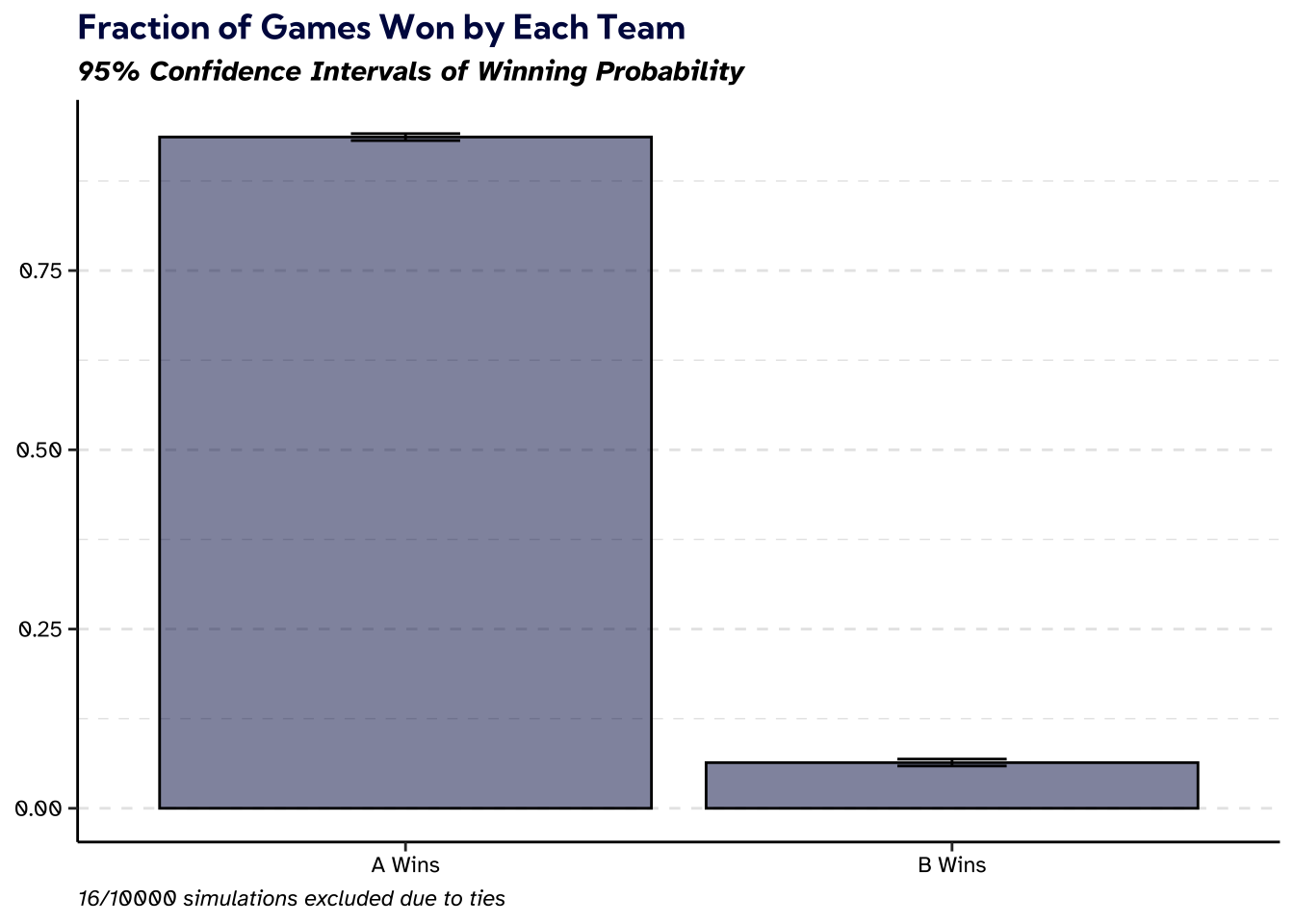

When team \(A\) does better in the first round, the figure makes it clear that the game is heavily tilted in favor of team \(A\). In such scenarios, the simulation reveals that team \(A\) wins more than 93.21% of games.⁴

An even more compelling way to visualize the disparity is with final scores. The plot below shows the final scores for both teams after team \(A\) is favored in the first round. Lighter areas are point totals that are more common. Completely blue areas are score pairs that never occurred. Values below the diagonal \(y=x\) line correspond to team \(A\) winning. If you’re familiar with the YouTuber John Bois, this is essentially a “scorigami” diagram for The Quiz With Balls.

counts <- 
  df |> 
  select(game_no, name, points) |> 
  tidyr::pivot_wider(names_from = "name",
                     values_from = "points") |> 
  summarize(n = n(), .by = c(A,B))

min_points <-  min(df$points)
max_points <- max(df$points)

possible_scores <- expand.grid(A = min_points:max_points,
                               B = min_points:max_points)

counts <- 
  left_join(possible_scores, counts, by = c("A","B")) |> 
  mutate(n = ifelse(is.na(n),0,n))


gg <- 
  ggplot(counts)+
  geom_raster(aes(x=A,y=B,fill=n))+
  geom_abline(aes(slope = 1,intercept = 0), col = "white")+
  geom_text(aes(x=45,y=47),
            label = "Team A Wins Below This Line",
            col = "white", angle = 45,
            family = "Atkinson Hyperlegible")+
  xlim(c(8,65))+
  ylim(c(8,65))+
  coord_equal(expand=FALSE)+
  xlab("Team A Final Score")+
  ylab("Team B Final Score")+
  labs(fill="Games", caption = glue::glue("From {nrow(df)/2} Simulations"))+
  theme(legend.text = element_text(color = "white"),
        legend.title = element_text(color = "white"),
        legend.key = element_rect(color="white"))+
  ggtitle("Distribution of Final Scores When Favoring A",
          "Thousands of Dollars")
gg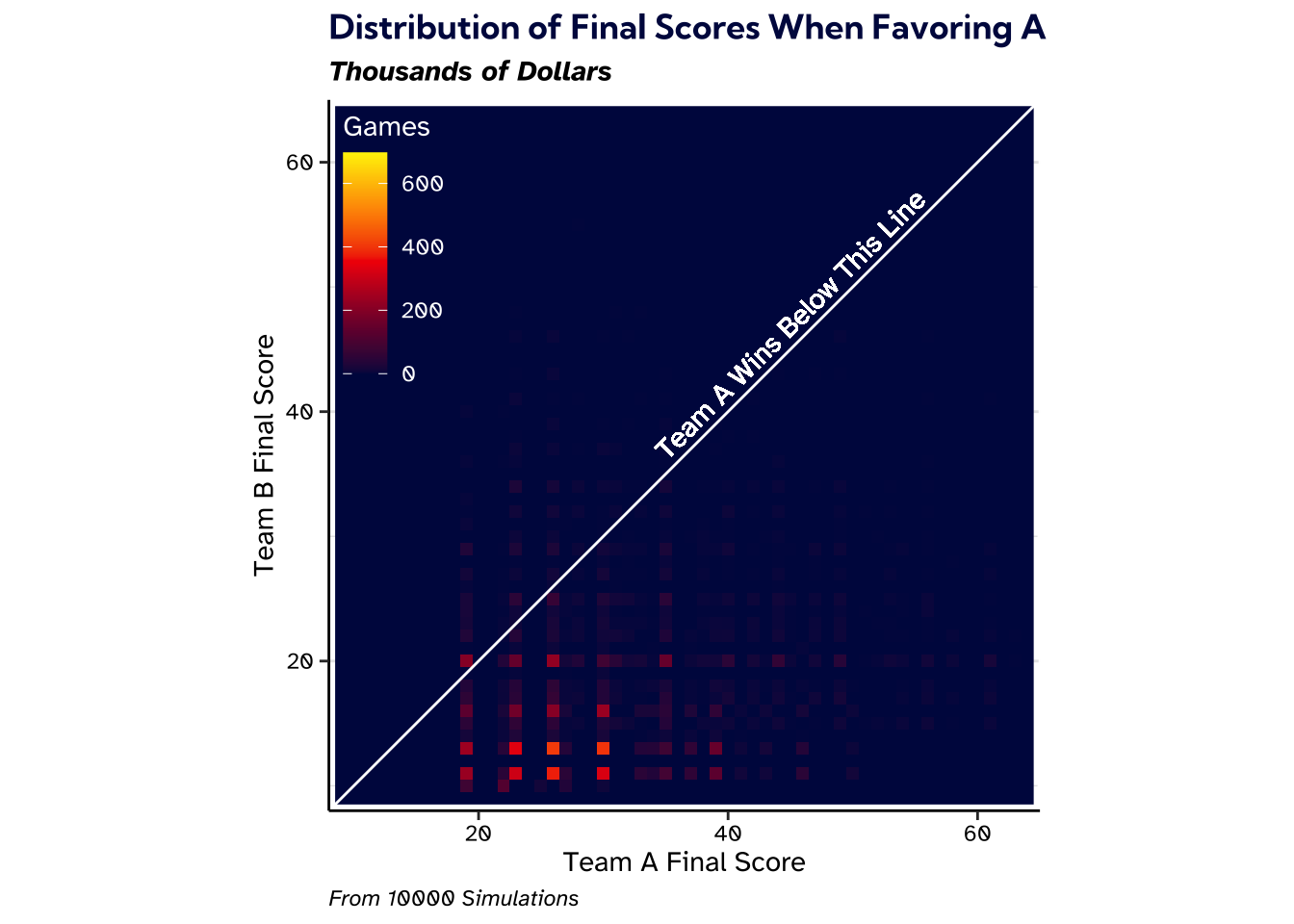

There is barely any light above the diagonal line which means that team \(B\) almost never scores more than team \(A\). The game becomes strongly biased in favor of the team that won the first round.

This also visualizes how complicated the scoring is for The Quiz With Balls. There are gaps between the lit up areas because certain point totals are impossible because of constraints on players and point multipliers.

Wrapping Up

An effective game show should keep the audience in suspense. Knowing the winner of an hour-long program at minute 10 is not ideal. The most likely outcome of the first round is both teams losing a player. However, there’s a 27.78% chance that one team is favored going into the second round. And in those cases, the winner is determined more than 93.21% of the time. So all in all, there’s a 25.89% chance that you will know the winner after the first round.

And if you’re empirically minded, we can look at the results of the actual show. Of the first 5 episodes (the only episodes available at time of writing), 4/5 games go into round 2 favoring one team. In all of those games, the favored team wins. In the other game, both teams lost a player in the first round. This sample is too small to trust, but it does provide initial evidence supporting my claim that the first round often determines the outcome.

Footnotes

1. Colors taken from here, here, and here.

2. There’s only ever \(6\) balls, but the \(b\) just helps to generalize the thinking.

3. There is a little bit of strategy when deciding which player to allocate to which answer, but usually the answers are so low confidence that we can reasonably model the players as randomly deciding on the answer.

4. 93.21% is the lower-bound of the 95% confidence interval of the one sided binomial test.