Quantitative Walking

Generating “Optimal” Walking Routes Using Graph Theory

Introduction

 

I have highly idiosyncratic preferences when it comes to my exercise routine. I like to walk or run outdoors in a closed loop of a pre-determined length with minimal backtracking on the same roads. In this post I develop an equally idiosyncratic algorithm to generate candidate routes for my runs. I incorporate ideas from graph/network theory and Geographic Information Systems to generate routes satisfying my criteria.

As with many problems in graph theory, finding truly exhaustive or optimal solutions is computationally challenging. In this post, I use a series of heuristics that allow me to generate desirable walking routes, even if they are imperfect.

The Road System as a Network

One way to view the road system in a given area is as a network where each intersection is a node, and the roads or paths connecting intersections are edges. In this framing, the term intersection is meant literally, any place where someone can change from one road to another is an intersection, regardless of whether or not there is a traffic light or stop sign.

Thankfully, the excellent OSMnx python package takes care of converting Open Street Map (OSM) geospatial data into python’s network handling package, Networkx (nx).

Below I have plotted an interactive view of the road network for some of Hibbing, Minnesota.¹

import os
import networkx as nx
import osmnx as ox
import geopandas as gpd
import numpy as np
import matplotlib.pyplot as plt
import itertools
import random
random.seed(1)

miles = 5

#https://ironrange.org/listings/bob-dylans-childhood-home/
center_coords = [47.42185416567268, -92.93401175307781]

def get_network(center_coords, miles_diameter, filepath = 'network.graphml'):
  if os.path.exists(filepath):
    G = ox.io.load_graphml(filepath)
  else:
    radius = 1609 * miles/2 # meters to miles
    G = ox.graph_from_point(center_coords, dist=radius, network_type="walk")
    ox.io.save_graphml(G, filepath)
  
  return(G)
    
    
G = get_network(center_coords, miles)  

my_house_gdf = gpd.GeoDataFrame(
    geometry=gpd.points_from_xy([center_coords[1]], [center_coords[0]]), crs=ox.settings.default_crs
)
x = my_house_gdf.geometry.values.x[0]
y = my_house_gdf.geometry.values.y[0]

my_node = ox.nearest_nodes(G, x, y)

coord_delta = .005

x_min = G.nodes[my_node]['x'] - coord_delta * 5/3
y_min = G.nodes[my_node]['y'] - coord_delta
x_max = G.nodes[my_node]['x'] + coord_delta * 5/3
y_max = G.nodes[my_node]['y'] + coord_delta

def in_bounds(G, n, x_min, y_min, x_max, y_max):
  node = G.nodes[n]
  if node['x'] < x_min:
    return False
  elif node['x'] > x_max:
    return False
  elif node['y'] < y_min:
    return False
  elif node['y'] > y_max:
    return False
  else:
    return True

subgraph_nodes = [n for n in G.nodes if in_bounds(G, n, x_min, y_min, x_max, y_max)]

G_subset = G.subgraph(subgraph_nodes)

node_gdf, edge_gdf = ox.convert.graph_to_gdfs(G)


import geopandas.explore
geopandas.explore._MAP_KWARGS += ["dragging", "scrollWheelZoom"]

m = edge_gdf.explore(
  color = "#000D4D",
  zoom_control=False, dragging=False, scrollWheelZoom=False,
  zoom_start = 13.5
  )
m = node_gdf.explore(m = m, color = "#55CE58")

m

Make this Notebook Trusted to load map: File -> Trust Notebook

Notice that some areas are very dense with nodes (intersections). This can happen when there are lots of intersecting foot paths. There’s also lots of very short edges, this can happen because every cul-de-sac, alley, and footpath should be coded as road.

If you hover over the roads in the above network it should tell you the length of each edge. Thanks to OSMnx, I don’t need to worry about the geocomputations to calculate a route’s total length, I can simply add up the length of each edge.

Formulating the street network as, well, a network allows me to use some ideas from graph theory to find routes that satisfy my criteria—but I should precise about what those criteria are.

Precisely Defining the Objective

Before I set out on a run or a walk, I usually calculate how long I have, and work backwards to calculate how long my route can be within my time constraints. For the purposes of this post, I’ll assume I’m looking to run \(D\) miles. However, I know that imperceptible changes to my route or stride might increase or decrease the total distance I travel, so I accept some imprecision, \(\varepsilon\). Specifically, I would like an algorithm that generates routes in the range of \([D-\varepsilon, D+\varepsilon]\).

The simplest way to run \(D\) miles would be to run \(D/2\) miles along any route, turn around, and run back on exactly the same route. This “out and back” is great because it ensures that you hit your target distance precisely. However, for me, the out and back feels repetitive. With this in mind, I aim to run in loops that don’t repeat edges in the graph.

Since edges are stretches of road, I aim to limit the number of repeated edges. I do not, however, try to minimize the number of nodes that I revisit. I can revisit the same intersection multiple times if at each visit, I choose a different path. There is no guarantee that a path with zero overlap exists. For example, if I lived in a house with a long driveway, I would have to run the length of that driveway coming and going—no matter the route that I choose. As such, I try to limit, but not eliminate overlap.

Finally, I like routes that take me somewhat far away from my starting point. One possible way fill the \(D\) miles would be to weave back and forth on every alley that’s near my starting point. This would fill my distance quota but would involve so many turns as to be dizzying. I prioritize routes that take me farther away from my starting point.

Of these three objectives, I deem hitting the target distance range to be most important. The method that I build will give guarantees on the total distance while aiming to (but not ensuring that) the other criteria are met.

A Heuristic for Creating Good Routes

I propose a heuristic route planner based on the ruler and compass construction of an equilateral triangle. To construct an equilateral triangle of perimeter \(D\) with starting at point \(A\), first draw a circle of radius \(D/3\) around the point \(A\).² Then, take any point \(B\) on the circle, and draw a new circle of the same radius (\(D/3\)) with \(B\) as the center. This will intersect the original circle in two places. Take either of those two intersections and call this point \(C\). The lines connecting \(A\) to \(B\), \(B\) to \(C\), and \(C\) to \(A\) must form an equilateral triangle. This is because the line segments were constructed using radii of length \(D/3\), and since the three sides form a closed loop, the triangle must be equilateral. The total length of this loop (the perimeter of the triangle) is \(D/3+D/3+D/3 = D\), the desired length.

If you’re more visually inclined, here’s a Desmos applet with the construction for you to play with. You can adjust the total route length by sliding the \(D/3\) segment. You can also adjust which point \(B\) you choose on the initial circle surrounding \(A\).

Triangles constructed in this way satisfy nearly all of the desired criteria. I can specify their total length ahead of time, there is no back-tracking, and the route ventures relatively far away from home. The triangle construction works so well for this purpose because the point \(C\) is guaranteed to be far—but not too far—from points and \(A\) and \(B\). Specifically, the only valid \(C\) are points a distance of \(D/3\) from both \(A\) and \(B\). If I choose an arbitrary point on \(B\)’s circle (i.e. not one that intersects with \(A\)’s circle), then it may be that our choice of \(C\) is much too far from \(A\) to return by the desired distance. Alternately, I might choose a \(C\) that is very close to \(A\), undershooting the desired distance. For these reasons, equilateral triangles are the way to go.

Of course, I can’t impose my triangles onto the geography of the real world. However, the process of constructing a circle of predetermined radius, choosing a point on that circle, constructing another circle of the same radius, and then looking for where they intersect generalizes nicely onto the graph structure that I have. I just need to define what a circle and radius mean in the context of the graph.

The Ego Graph

In graph theory, an ego graph of radius \(D/3\) takes a node \(n\) as an input and returns all other nodes, \(n'\), such that distance from \(n\) to \(n'\) is less than \(D/3\).³ This is a natural generalization of a circle—all points a distance \(D/3\) away from a given point. However, in the context of the graph I do not mean the Euclidean distance. Here distance will mean the sum of the distances along each edge from \(n\) to \(n'\).

Below I have plotted an example of an ego graph:

def get_ego_disc(G, origin_node, target, tol_lower, tol_upper = None, weight="length"):
  if tol_upper is None:
        tol_upper = tol_lower

  nodes = nx.single_source_dijkstra_path_length(G, origin_node, cutoff = target+tol_upper, weight = weight)

  return nodes

disc_nodes = get_ego_disc(G, my_node, 1609 * 1, 0)

def color_map(node, disc_nodes, my_node):
  if node == my_node:
    return("#FF00FF")
  elif node in disc_nodes:
    return("#55CE58")
  else:
    return("#375237")

def radius_map(node, disc_nodes, my_node, k = 3.0):
  return(60/(k**2) if node == my_node else 7.5/(k**2))

node_gdf, edge_gdf = ox.convert.graph_to_gdfs(G)
node_gdf['id']=node_gdf.index.values

import geopandas.explore
geopandas.explore._MAP_KWARGS += ["dragging", "scrollWheelZoom"]

del m
m = edge_gdf.explore(
  color = "#000D4D",
  style_kwds = {"opacity":.3},
  zoom_control=False, dragging=False, scrollWheelZoom=False,
  zoom_start = 13.5
  )
  
  
m = node_gdf.explore(
  m=m,
  style_kwds={
    'style_function':lambda x: {
      "color":color_map(x["properties"]["id"], disc_nodes, my_node),
      "fillOpacity":1,
      "fillColor":color_map(x["properties"]["id"], disc_nodes, my_node),
      "radius":radius_map(x["properties"]["id"], disc_nodes, my_node)
      }
    }
  )
  
m

Make this Notebook Trusted to load map: File -> Trust Notebook

The large magenta point represents the origin point, \(A\), around which the ego graph was drawn. The bright green points represent intersections that are \(D/3\) miles or shorter from the origin. The darker nodes on the exterior represent points that cannot be reached in \(D/3\) miles or less. The light green area is highly irregular. Some areas that are close in Euclidean distance are not in the ego graph. Such points are hard to navigate to from the origin point because of inconsistencies in the road network.

While the previous section relied on circles, technically the map above is a disk. The map above contains points very near to the origin, not just points on the circle exactly \(D/3\) miles out. To adapt the methodology from the previous section, I should restrict the disk to instead be a thin doughnut of points that have distance in the range of \([D/3 - \varepsilon/3,D/3 + \varepsilon/3]\).

Updating the map to reflect this change gives:

def get_ego_doughnut(G, origin_node, target, tol_lower, tol_upper = None, weight="length"):
  if tol_upper is None:
        tol_upper = tol_lower

  nodes = nx.single_source_dijkstra_path_length(G, origin_node, cutoff = target+tol_upper, weight = weight)
  nodes = [k for k,v in nodes.items() if v >= target-tol_lower]

  return nodes

doughnut_nodes = get_ego_doughnut(G, my_node, 1609 * 1, 1609 * 1 * .1 / 3)

def color_map(node, doughnut_nodes, my_node):
  if node == my_node:
    return("#FF00FF")
  elif node in doughnut_nodes:
    return("#55CE58")
  else:
    return("#375237")

def radius_map(node, doughnut_nodes, my_node, k = 3.0):
  if node == my_node:
    return(60.0/(k**2))
  elif node in doughnut_nodes:
    return(30.0/(k**2))
  else:
    return(7.5/(k**2))

del m
m = edge_gdf.explore(
  color = "#000D4D",
  style_kwds = {"opacity":.3},
  zoom_control=False, dragging=False, scrollWheelZoom=False,
  zoom_start = 13.5
  )
  
  
m = node_gdf.explore(
  m=m,
  style_kwds={
    'style_function':lambda x: {
      "color":color_map(x["properties"]["id"], doughnut_nodes, my_node),
      "fillOpacity":1,
      "fillColor":color_map(x["properties"]["id"], doughnut_nodes, my_node),
      "radius":radius_map(x["properties"]["id"], doughnut_nodes, my_node)
      }
    }
  )
  
m

Make this Notebook Trusted to load map: File -> Trust Notebook

The remaining bright green nodes are the potential valid choices for \(B\). Now, I should draw similar doughnuts around each \(B\) and see if I can find any points, \(C\), that are within the donuts of both \(A\) and \(B\). If such a point exists, then I am guaranteed the distance along all three legs is in the target distance range of \([D-\varepsilon, D+\varepsilon]\).

In practice, I do this for every possible \(B\) so I can find all possible triangles, but here is the overlapping doughnuts for one \(B\):

Cs = {node:get_ego_doughnut(G, node, 1609 * 1, 1609 * 1 * .1 / 3) for node in doughnut_nodes}

intersections = {k:[n for n in v if n in doughnut_nodes] for k, v in Cs.items()}
intersections = {k:v for k,v in intersections.items() if len(v) > 0}

# Compute the B that has the most possible C's
most_overlap = 0
for k, v in intersections.items():
  if len(v) > most_overlap:
    most_overlap = len(v)
    best_B = k
    
def triad_color_map(node, a, b, a_doughnut, b_doughnut, intersection):
  if node in [a, b]:
    return("#FF00FF")
  elif node in intersection:
    return("#6D55CF")
  elif node in a_doughnut:
    return("#55CE58")
  elif node in b_doughnut:
    return("#CF8B55")
  else:
    return("#375237")

def radius_map(node, a, b, a_doughnut, b_doughnut, intersection, k = 3.0):
  if node in [a,b]:
    return(60.0/(k**2))
  elif node in intersection:
    return(60/(k**2))
  elif node in a_doughnut + b_doughnut:
    return(30.0/(k**2))
  else:
    return(7.5/(k**2))
  
m = edge_gdf.explore(
  color = "#000D4D",
  style_kwds = {"opacity":.3},
  zoom_control=False, dragging=False, scrollWheelZoom=False,
  zoom_start = 13.5
  )
  
m = node_gdf.explore(
  m=m,
  style_kwds={
    'style_function':lambda x: {
      "color":triad_color_map(x["properties"]["id"], my_node, best_B, doughnut_nodes, Cs[best_B], intersections[best_B]),
      "fillOpacity":1,
      "fillColor":triad_color_map(x["properties"]["id"], my_node, best_B, doughnut_nodes, Cs[best_B], intersections[best_B]),
      "radius":radius_map(x["properties"]["id"], my_node, best_B, doughnut_nodes, Cs[best_B], intersections[best_B])
      }
    }
  )
  
m

Make this Notebook Trusted to load map: File -> Trust Notebook

In the plot above, the pink nodes represent \(A\) and \(B\). The green nodes, as before, represent the doughnut surrounding node \(A\). The orange nodes represent the doughnut surrounding node \(B\). However, the larger purple nodes represent where the green and orange overlap. These purple nodes are possible choices for \(C\), completing our triangle! Any of the purple \(C\) will be within the desired total route tolerance, I can choose one at random, or be more selective about which one produces the optimal route.

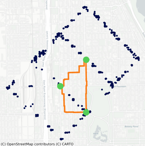
Now, all that’s left is to actually compute the path from \(A\) to \(B\) to \(C\) then back to \(A\). This task is also easily completed with OSMnx.

C = intersections[best_B][0]

A_to_B = ox.shortest_path(G, my_node, best_B)
B_to_C = ox.shortest_path(G, best_B, C)
C_to_A = ox.shortest_path(G, C, my_node)

full_route = A_to_B + B_to_C[1:] + C_to_A[1:]

route_length = sum(G.edges[i,j,0]['length'] for i, j in itertools.pairwise(full_route)) / 1609
route_length = round(route_length, 2)

triangle_gdf = node_gdf[node_gdf['id'].isin([my_node, best_B, C])]
route_gdf = ox.routing.route_to_gdf(G, full_route)

m = route_gdf.explore(
  color = "#55CE58",
  style_kwds={"weight":5},
  zoom_control=False, dragging=False, scrollWheelZoom=False,
  zoom_start = 15
  )
  
m = triangle_gdf.explore(
  m=m,
  style_kwds={
    'color':"#FF00FF",
    'fillColor':"#FF00FF",
    'fillOpacity':1,
    'radius':60.0/9
    },
  )
  
m

Make this Notebook Trusted to load map: File -> Trust Notebook

The above route does a good job of meeting all of my criteria. I was targeting a total length of \(D=3\) miles with an \(\varepsilon=0.1\) miles, and the resultant route is 2.94 miles—well within the specified tolerance. The route is also definitely not an out-and-back. The route has minimal backtracking and repeated edges. Finally, this route also manages to travel relatively far away from home.

Of course, I arbitrarily chose \(B\) and \(C\) from the valid options, but other valid choices result in different desirable routes. This technique is definitely a heuristic because it provides no guarantees about the amount of overlap or back-tracking, but so long as the road network is sufficiently dense, it tends to do a good job while ensuring the target distance is hit. Applying this technique to where I live gives even better results due to the increased density of roads.

Limitations and Extensions

If you stare at the above route for long enough, you will notice that there are short portions of the route that backtrack. These sections of backtracking occur when the path from \(A\) to \(B\) ends the same way that the path from \(B\) to \(C\) starts. You can easily trim these repeated portions off, but you are no longer guaranteed to hit the target distance band. One possible solution is to attempt to trim off the overlap, but if the total distance moves out of the desired range, accept the overlap.

I originally came up with this method so that I could generate many routes and randomly sample from them to give me the route I should run that day. My first instinct was to look at every possible \(B\) and \(C\) combination that formed a valid triangle with \(A\) and sample from all such triangles. This turns out to be a bad idea. If you naively sample from the distribution of triangles, you might find that 90% of routes look very similar. This can happen if there are some areas of the map that are very dense with nodes (say dense residential blocks). If two of these dense areas happen to be a distance of \(D/3\) away, then this can generate a ton of triangles because the number of triangles formed by those two clusters increases multiplicatively. Really what I want is to sample over the distribution of substantially different triangles To do this, I use Louvain community detection to identify which nodes are very similar to one another and group them into communities. Then I look for the distinct triangles between communities (instead of between individual nodes). Since communities are designed to be different from each other, if two triangles pass through different communities, I can be more confident those routes will feel qualitatively different.

This method also cannot distinguish walkable roads from car-only roads. This method might propose you run on a 60 mile per hour road with no shoulder or sidewalk. With local knowledge, one can exclude certain edges from the road network graph, but this has to be done on an ad hoc basis.

The proposed algorithm often takes the shortest route between two points. This is useful to give distance guarantees but has two potential annoyances. First, if you’re planning to run on a street grid, and you are trying to run diagonally to the grid, the algorithm may recommend that you go up one block, over one block, up one block, over one block, and so on. A human runner might prefer to go up \(n\) blocks, then over \(n\) blocks, minimizing the number of required turns. It would be up to the runner to determine if this is appropriate in their context. Additionally, the proposed routes use distance, not actual travel time. This means that the algorithm may propose a route that goes through many traffic lights which might annoy runners who wish to keep a consistent pace. To help with these problems, one could score routes after generating them to figure out which routes have the fewest turns.

Finally, this algorithm currently does not incorporate any information about elevation changes. It might tell you to run up a mountain so long as there’s a walking path. This may not be desirable. OSMnx has the ability to incorporate elevation data, but I’ll save that for another day.

There are many more nitpicks and extensions you could make to this model, but problems in graph theory are hard, and good-enough heuristics are often good enough. This technique has been useful to me personally to generate new routes I wouldn’t have otherwise discovered.

Footnotes

1. I chose Hibbing Minnesota for two reasons. First, I didn’t want to give away my precise home location. Second, it’s purported to be Bob Dylan’s hometown.

2. Trisecting a line segment of length \(D\) using a ruler and compass is non-trivial. See Tim Lehman’s post for an explanation.

3. There may be multiple ways to reach a given \(n'\) from \(n\). When constructing the ego graph, if there exists any path with distance less than \(D/3\) I include \(n'\) in the output.